By Gerard Gilliland
I originally presented this subject at an Instrument Society of America (ISA) seminar in Denver in the spring of 1991. Although these graphics reflect the overhead projecter that I used back then and today’s simulation software (20 years later) consists of drag and drop libraries, I still think this paper is useful as an introductory background and for simulation concepts.
Purpose:
The purpose of this seminar is:
1) To introduce simulation: It will provide you an opportunity to learn some of the lingo. In addition, I hope to stimulate your interest in simulation.
2) To show that simulation can provide savings in design, testing, training, and production. However, the element of cost has another side as well. Thus, I hope to provide you with concepts that need to be analyzed before committing to a simulation specification.
3) To give a realistic viewpoint of what is achievable today. That is, this paper should balance the two opposing viewpoints:
"Simulation can solve all my problems. -- dream on”
"Simulation can't do anything meaningful or useful -- wake up"
A manager at a major research center made a million dollar mistake. He went in to give his resignation but his management wouldn't accept it. "What? You can't leave now. I've just invested a million dollars in your education." Perhaps YOUR management wouldn't be quite as understanding, ...but there may come a point in your life when your simulation supplier rubs his hands together and asks "Oh!... You want it to run too?" In other words... I intend to present "things to think about before signing on the dotted line."
There are two major types of simulation: Stochastic and Deterministic.
Stochastic
The definition for Stochastic is -- event stepped simulation.
Stochastic simulation represents the required sequence of activities in a system. It shows where activities may proceed in parallel and where coordination between activities is required.
Figure 1: Petri Net
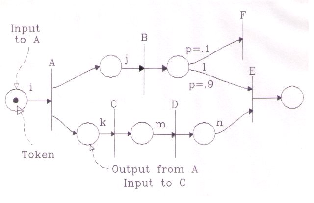
Figure 1 shows a simple petri net. This is similar to a Program Evaluation Review Technique chart, more commonly known as a PERT chart.
The vertical bars are called transitions. They represent activities. These transitions are labeled with capital letters.
The circles are called places. They represent the inputs and outputs of the transitions.
The lines show the flow through the network.
The 'action' of the network is dependent on the availability of the 'inputs' to each activity.
This availability of an input is represented by a 'token', (a black dot), in an 'input' 'place.' When all required inputs to an activity are available, the activity can continue; Or in Petri net lingo: "the transition is enabled and it 'fires.'"
When a transition fires it removes one token from each of its input places and places one token in each of its output places.
The existence of these outputs enables other transitions, and the activities can propagate through the network.
The basic concepts can be extended to include a timing rule. This rule models the length of time required to complete the activity. This timing rule is usually defined by random distribution. Some simulations call for linear or exponential distribution.
The class of situations can be extended by introducing branches into the network. In this example, a situation can exist where activity B produces an output that can be an input to either E OR F. Now E and F are in conflict. If E fires, F cannot or vice-versa.
The conflict is resolved by assigning a decision rule to the activity where the conflict occurs. In this example, there is a decision rule based on probability: the token will branch to transition F with probability 0.1 and to transition E with probability 0.9. Scarcity of resources is typically resolved in this manner.
Other rules can include situations where an activity cannot start without the presence or absence of some other factor which is not itself an input to (that is, used up by) the activity. These rules can be inhibiting or enabling. For example, customers could line up in a queue for a particular service but could not be admitted if the door is locked.
Examples of Stochastic simulation include: Petri nets, maintenance scheduling, PERT charts, just-in-time production, and line queues.
This in summary is Stochastic simulation -- or event stepped simulation.
Deterministic
The second major type of simulation is Deterministic.
This is a simulation that can be described mathematically.
A typical simulation can include simple algebraic equations, Boolean logic, and time dependent non-linear ordinary differential equations.
Examples of deterministic simulation include aerospace dynamics, chemical reactions, automotive dynamics, power plants, robotics, control systems, and biomedical research.
Since I am more familiar with deterministic simulation, the rest of this discussion will focus on this second type of simulation. However, obviously both types of simulation can and do occur in the same program. Mechanical faults and failures can occur at any random time, and their faults can propagate through the system. Electrical timer circuits, hand switches and contacts can enable or disable the deterministic simulations.
Figure 2: Typical Electrical Circuit
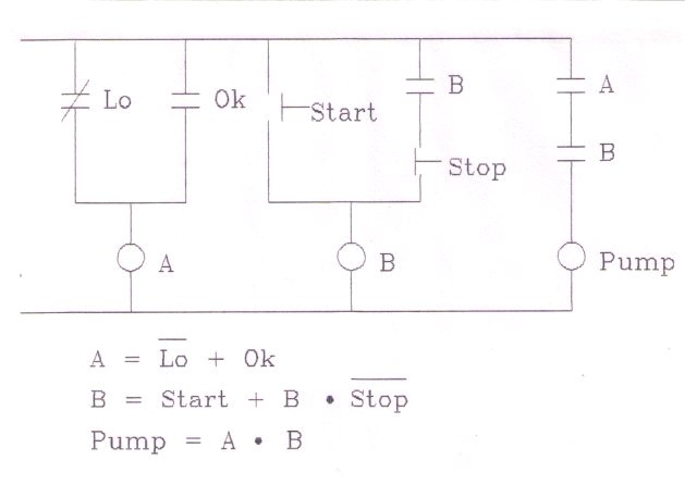
Figure 2 is a typical electrical circuit where relay A is true -- energized -- when either NOT Lo OR Ok is true.
Remember two rules: the prints are always shown de-energized and -- George Boole used Plus signs for OR and Dots for AND.
Path B is described as "Start OR B AND NOT Stop."
And finally, the Pump will run if both conditions A AND B are true.
Simulation vs. Modeling
I've talked about simulation and modeling. What is the difference?
Simulation is the process that provides a synthetic environment to test, evaluate, design, change, or create a real-world concept. (The forest)
Model by definition is the translation of a real-world concept into a computer duplicate-able code. (The trees)
Definitions
Let's continue with some more definitions.
General requirements:
Out of one list -- and into another -- sorry about that.
At this point I'll list several requirements that most simulation projects will need to be successful.
Design requirements:
The most difficult question to answer is: How much is enough? This question must be asked in the areas of financial investment, alcohol consumption, and simulation. -- or -- You have to "know when to say when."
Thus "Extent of simulation" needs to be capitalized and underlined and circled in red.
You could say, I'll model the states of this hand switch. Or you could say, I'll include the contacts in the hand switch. The next thing you know is you're including pull to lock, spring return to normal, and rust on the nameplate.
I'll bet hard money that "Extent of Simulation" has killed more simulation projects than all other reasons combined"
"Extent of simulation"
"How much is enough?"
"Know when to say when"
Some External factors include Location of simulation. Will it be "built" or "coded" on site or at a remote location? What site requirements will need to be added or modified? Will you need expanded electrical capability, lighting, HVAC. (not so much for the equipment anymore but for the added personnel)
Performance Requirements:
Simulation is a "hog" as far as timing and memory requirements go, and a math co-processor is almost mandatory.
Although vague, the subject of Performance needs to be addressed. You need to know how many frames per second you can expect out of your simulation. Depending on your answer to "How much is enough?", this may or may not be important. If you plan to run real-time simulations, look at your transient operations data to see the worst case scenario of the thru-put you will need. Performance can be successfully degraded if you only intend to run steady-state operations. Real-time simulations can be run slower than real-time and accurately reflect all parameters except time. The basic question to ask is "What performance do you want from transient operations, normal evolutions such as startup and shutdown of the reference), and what performance effect will malfunctions have?"
Other design considerations include Manual operations, which we learned earlier is "Input of signals / data outside the boundary.", and Initial conditions. Do you need to start the simulation from all conditions?
Languages:
There are as many simulation languages out on the market as there are PhDs in computer science and engineering. Most simulation languages are typically a high level language -- a macro that gets compiled into Fortran. The current development is toward object oriented languages and improved human machine interface.
Software Functions:
Given our background now we can simply list the software functions that a simulation language should include:
Design Approach:
I'll cover design data in a little bit.
The Distributed / isolated / independent options is another way of asking if you are going to run on more than one computer and share the data.
First principle modeling is nearly always used (and is highly recommended). This is the conservation of energy, and mass. If you don't use first principle modeling you'll disappoint yourself and Sir Isaac. You'll also violate the second principle and find that your simulation project that is supposed to be moving will come to rest.
Software requirements:
Simulation spans several systems. That is, the simulation language is just a part of the total system. This may be the second most popular cause of simulation failure, and has nothing to do with simulation. That is, you can get bogged down in making the other parts of the system work: Learning the operating system, making files shareable, etc.
Thus software requirements include:
Look for Open Systems Interconnect and compatibility. You might have the two neatest packages in the world, but if they need to share data and they are not compatible they're not worth the shrink wrap they came in.
Inspection:
The following items are the "Packing lists" for a simulator project. That is, If you are buying a simulator, when you open up your simulator box, this is what you should find inside:
Documentation:
Hardware documentation should include:
Software documentation includes:
Note: The next 9 drawings (from Select the System (Step #1a) to Define the Control System (Step #4)) came from EPRI MMS "Building A Model" (see References below.)
Now we come to the simulation process: This is process or procedure needed for developing a model.
Step #1: Select the system:
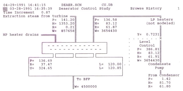
For this session, we'll use the development of a deaerator level control system. You can see a typical low pressure heater train.
Figure 3-1a: Select the System
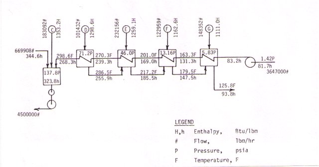
Figure 3-1b: Draw the Model Schematic
This is a simplified process schematic showing all components to be modeled. Define the boundaries.
The scope and limitations of the simulation are already apparent: the model cannot be used for feedwater heater studies.
Step #2: Draw the Interconnection schematic.
Figure 3-2: Interconnection Schematic
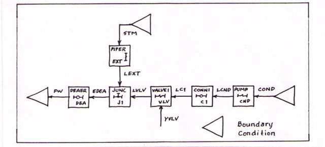
The interconnection schematic is a reconstruction of the Model Schematic (Figure 4) using the modeling system libraries. Before you can do this you need to know what libraries exist or if you are a masochist what libraries need to be written.
Step #3: Parameterize the model
This step consists of calculation or definition of all constants and initial conditions for each module in the interconnection schematic.
Parameterization is the most complex and time consuming step in the model generation process. All other steps are measured in minutes or hours while this step is measured in days or weeks.
The primary objectives are to arrive at reasonably accurate parameters for each component in the model and to define the model initial conditions accurately enough to bring the model to an initial steady state.
The calculations are made using the same equations used in the model during simulation, but transposed to solve for the coefficients. For example, the equation in Figure 3a is used to solve for flow in a pipe module:
Figure 3a: Parameterize the Model
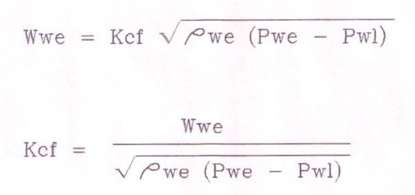
You transpose the equation to solve for the conductance off-line using steady-state operating point data:
You collect the module physical data from: Field data, the preferred source of information, or from Vendor component design data, or ... the least preferred System design data.
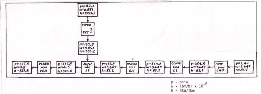
Step 3b: Draw parameterization schematics(s) and collect operating point data. These data are used to calculate the heat transfer coefficients and flow conductances in many modules. Compare Step 3b below with Step 2 above. It is the same schematic with Pressure, Flow and Enthalpy added between each module.
Figure 3b: Parameterize the Model
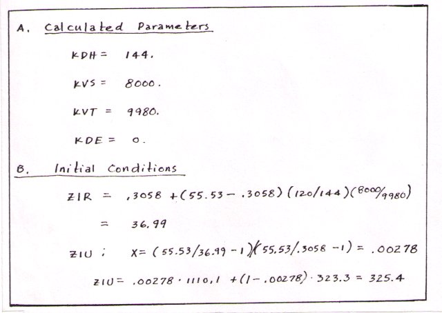
In steps Step 3c thru 3e you Calculate Module parameters and Initial conditions.
Two modules are shown here the extraction piping and deaerator.
Figure 3c: Parameterize the Model
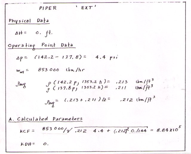
Figure 3d: Parameterize the Model
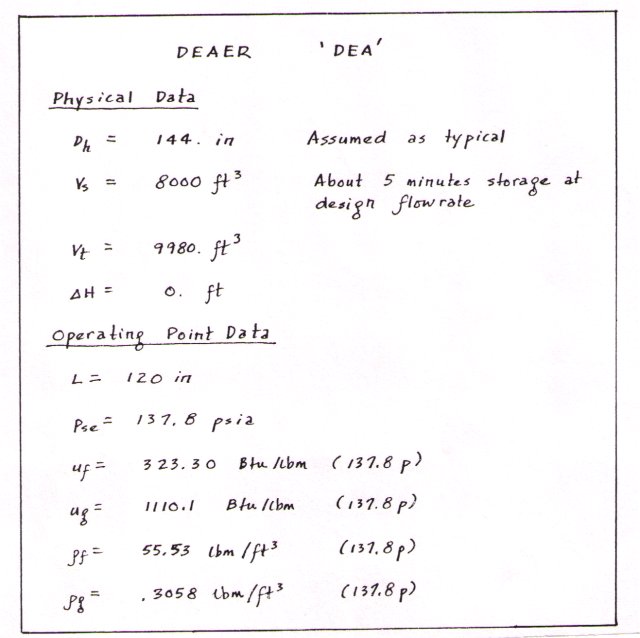
Figure 3e: Parameterize the Model
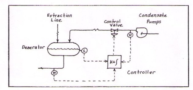
Step #4: Define the Control System
Figure 4: Define the Control System
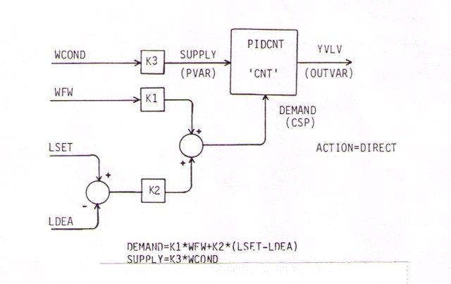
The control system for use with this model is defined to be a 3-mode controller. If you don't know "when to say when", the electrical schematics will be modeled using Boolean algebra (See Figure 2).
The process is continued until each model in the Interconnection Schematic (back in step 3b) is completed with data from the parameterization and control system definition.
Step #5: Code the Model
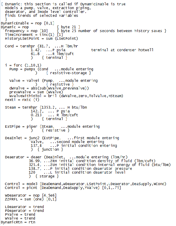
The model is coded according to the simulation library requirements. This is simply transferring the parameters into the format required by the library. Note: only the first two pages 5a-5b are input by the model builder.
Figure 5a: Code the Model
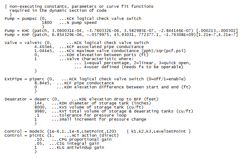
Figure 5b: Code the Model
Figures 5c-5f are included only for completeness. They are part of the module library, and are transparent to the model builder. But you have the option of building your own libraries if desired.
Figure 5c: Code the Model
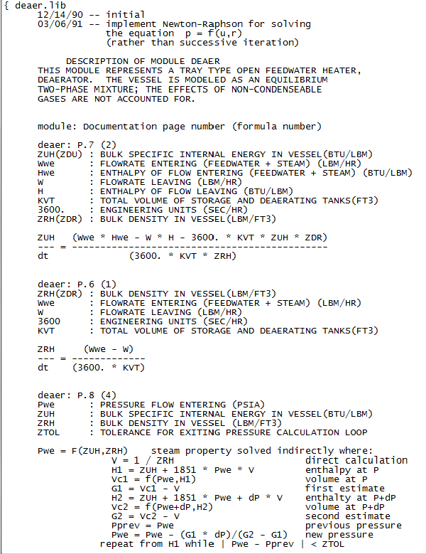
Figure 5d: Code the Model
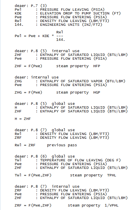
Figure 5e: Code the Model
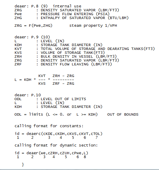
Figure 5f: Code the Model
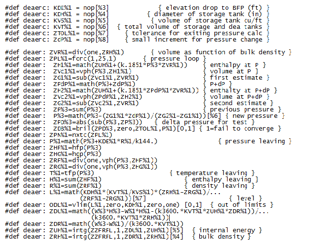
Figure 5g: Generate Executable Program
In Step #5g, the program is translated and compiled using the appropriate commands for the computer and software ... AND voila, a computer simulation.
Step #6: Comparing Integration Techniques.
Integration techniques: Gear (stiff) vs. Euler (differential equations)
At this time we need to analyze the different integration techniques and look at the analysis of large and small time steps. A system is "stiff" when there is a large difference between measured parameters. For example, you change flow several thousand pounds per hour to see a small change in pressure. Pressure changes very rapidly whereas temperature moves very slowly. The combination results in a "stiff" system.
Gear (another PhD), devised an integration technique for taking small steps when the system was changing rapidly and taking large steps when the system was steady. This is great for keeping down "runtime" costs on a mainframe, but it destroys real-time simulation. Euler, on the other hand, chugs along at the same steady rate. The smaller the step, the better the resolution, and the longer it takes.
As a solution to this dilemma, you can modify a dynamic simulation to run steady state.
Steady-state is -- the reference is faster than the simulation frame. For example, to answer the question "What transient pressures occur during pump start up?"
Use algebraic equations.
Dynamic -- The reference is slower than the simulation frame. For example: "What's the heater temperature going to be an hour from now?"
Use Differential equations (Euler).
Some equations will be steady-state, others will be dynamic. The typical simulation will be a combination of the two. This is the real world.
Figure 6a is Euler at his best. It has a time stamp of 10 milliseconds (ms). Use this as the baseline. If your simulation is unstable, run it with small time steps. If it's still unstable, you've got logic problems. If it becomes stable you may need to convert some dynamic equations to steady state.
Figure 6a: Euler at 10 ms
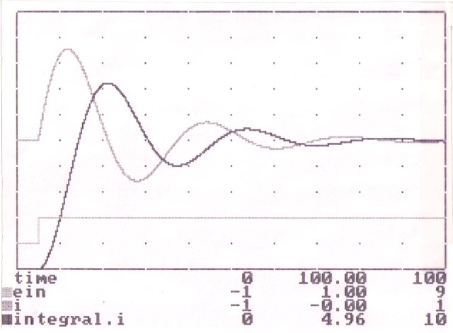
Figure 6b is labeled "real-time" in that it takes 100 seconds to draw this graph, regardless of the computer it runs on. Recognize that the real-time algorithm simplifies coding. You can use controller settings for proportional and integral directly from field data, and you don't have to modify code if you upgrade your computer. The time step is the time it takes to complete one pass through the code.
Figure 6b: Real-Time
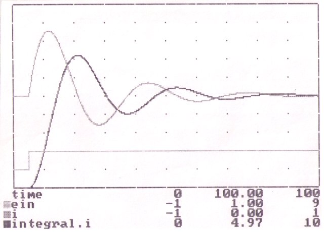
The next three figures show the real-time integration compared to Euler. Note that the real-time algorithm maintains a very valid amplitude compared to the baseline. However, all is not perfect. There is a small phase shift from the baseline. Standard Euler, falls apart at larger intervals (Figures 6d and 6e). And real-time (Figure 6c) will have the same result if it takes too long in each loop compared to the Euler baseline.
Figure 6c: Real-Time vs. Euler at 10 ms.
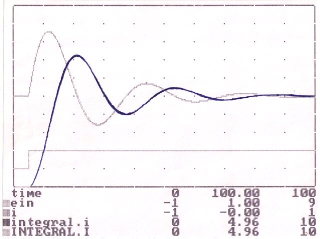
Figure 6d: Euler at 500 ms. steps vs. Euler at 10 ms.
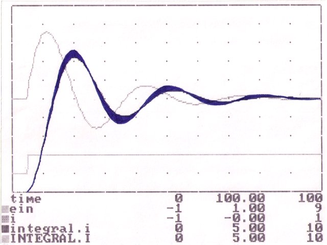
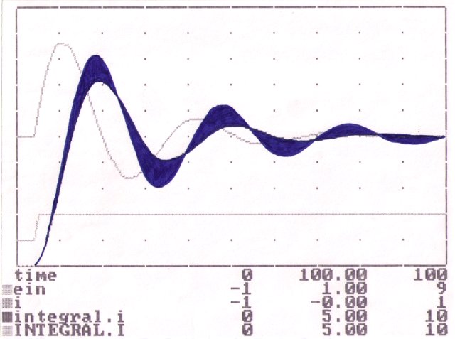
Figure 6e: Euler at 1 second steps vs. Euler at 10 ms.
AI Directions:
Combination Systems:
Now let's look beyond simulation by building a combined simulation / knowledge base / filter / expert system.
First we need a reality check.
Artificial Intelligence is not a "Popular terminology". If you want to kill a project, call it Artificial Intelligence. There have been many advances in our understanding of "Natural" intelligence. But this understanding hasn't had any effect on the acceptance of "Artificial" intelligence as a practical approach to solving "real world" problems.
The basic problem with the acceptance of most AI techniques is that they are seen by the user as un-provable.
The end users of AI want a clear explanation of the detailed operation of the system. They want a description of the underlying cause and effect that guides the operation. And they want some assurance of its correctness and completeness. "Successful" AI applications have been able to meet these requirements.
Expert Systems:
Expert systems are a good example. These systems only became viable when they began to provide a straight-forward explanation of their operation. The logic could be expressed in simple if-then phrases.
The more successful applications have been based on "deep" rather than "shallow" knowledge of their cause and effect.
The use of certainty factors associated with the results has bypassed the user's request for proof by emphasizing the "fuzziness" of the results, and by including a measurement of their correctness and completeness.
Knowledge-Based Systems:
The current emphasis is on "Knowledge-Based Systems" as a step beyond Expert Systems. I'm not sure if the difference is the increased complexity or if its Marketing.
The most successful knowledge-based systems are using representations which accurately reflect the way their users think about the particular subject matter. They include graphic "icons" to display the results in a way that seems "natural" to their users.
The use of special-purpose robots in factory automation is another example of the successful employment of AI technology. It is very reliable and its correctness and completeness can be proven by direct observation by knowledgeable humans.
The standard method of "teaching" (programming) robots is by having a human walk them through the process. This also serves to increase the human's confidence in the robot's operations.
Natural Languages:
The "Natural Language Interface" has not been as universally accepted as it was expected a few years ago. The present technology is actually quite reliable when used in relatively limited areas, such as queries against a database. However, there are always a few situations in which the interface reacts with apparent stupidity. And there are other cases where greater accuracy on the part of the user is required to achieve a successful outcome.
Natural language interfaces tend to be favored by occasional or beginning users. Such a user feels comfortable and confident in dealing with it. Once the user has reached a certain degree of familiarity with the system, he prefers to use a more compact and precise shorthand.
The interface can handle this style of interaction, but it doesn't require the AI technology that makes the interface more costly to build and less efficient to operate.
The well trained user feels he understands the system better than the interface does. The end result is he no longer trusts its correctness and completeness.
Neural Networks:
Technically, the next area of AI that appears ready for commercialization is that of Neural Networks.
This technology has the potential for solving a variety of problems. Among these are pattern recognition, discrimination of electronic signals, and maintenance scheduling. It can solve problems far more efficiently than is possible by any other means.
In some cases (such as optimum routing), the other means are so expensive or time consuming that there is no practical way to check the solution of the neural network for correctness and completeness.
The neural network doesn't use or generate any underlying cause / effect model, nor does it provide any detailed explanation of the operations it used when arriving at a particular result. Neural network people say their product is like a human brain. Dissecting it will not reveal the logic it used. However, humans are generally able to describe the logic (or at least the rationale) behind their decisions and actions.
Without the existence of cause and effect, the only way we can establish confidence is by a number of actual trials. The number of trials required is dependent on how unusual the solution seems.
To be commercially successful, a neural network application needs to establish user confidence in its result. If this can't be done by the neural network itself, then it needs be done by comparing the answers with some standard.
If we want the neural network to retrieve information from a very large database, its actual output can be judged for correctness, but a test of its completeness would require an exhaustive search. This is what we are trying to avoid.
If we want the neural network to control a process (say a chemical plant or a radar system), we could compare its results with an expert human or an existing conventional control system.
To reduce expense, time and potential danger, we can use a previously validated simulation of the process at least for initial testing.
Expert System Summary
All of this discussion is summed up as the basic problem of all expert systems:
Without some method for explaining its logic or quickly testing its results,
it takes as long for users to have faith in them as to have faith in an expert.
Recognizing this, let's begin with some definitions:
Expert system technology: A specific type of knowledge-based program that manages the expertise of a human. You know you're in trouble when the definition contains the word being defined. ... But let's try anyway.
Knowledge Base Definitions:
I was involved with the Colorado University on a system that used a combination data-acquistion, simulation and knowledge-base that explored "Fault Diagnosis in Dynamic Systems Using Analytical Redundancy." You can read that as an application of Kalman filters. The concept was use software combined with hardware to look for faults in the system. Fault tolerance can be achieved with hardware redundancy where repeated hardware elements are used: duplicate pressure, temperature and flow elements. But you would still not know the flow conductance, its deviation from normal, or what normal should be. Analytical redundancy is combining Quantitative knowledge (the mathematical properties of the system) and Qualitative knowledge (the expert's compiled knowledge in the form of rules and hypotheses). The tasks included: early instrument fault detection; abnormal operation of equipment; interpretation and prediction of plant performance for the evaluation of alternative operation and maintenance strategies.
Justification of simulation:
When planning a simulation project, ones finances and time obviously need to be justified. The following are some points to consider when working up the justification.
It can be (and has been) simulated: I will not attempt to list the areas of simulation: almost anything that can be described can be simulated. Look around in the industry to find similar projects. See how they justified their simulation and look at the approach they took.
Risk: The more successful simulation projects seem to be in the areas of greater risk: war games, flight simulators, Nuclear reactors, and financial markets. Is your life or wallet at risk?
Uncover complexity: The justification of simulation has often come after major rework. That is, the simulation could have more than paid for itself had it been implemented before the project started rather than after the engineering design proved faulty. Look at past projects and see if simulation would have uncovered the complexity. The savings would be proportional to the design complexity of the project.
Understanding and identification: Eliminate design duplication. Check for proper fault paths. The ability to fail any part of the circuit or system and see the results.
Identify the problem areas. Visualize where the problem is.
Cut down on rework: We have all seen pictures of an individual describing a need to an engineer, the engineer designing a different piece of equipment, and construction making something else totally different. Rework is a major cost.
To demonstrate that the change is actually needed: For example, a high pressure separator tank level control system, being modeled for understanding, cycled. Upon touring the real-world it was cycling as well.
On the other hand, a rotational drive was causing problems and a recommendation was made to replace it. After further study and simulation of the drive as part of the system. It became apparent the drive was doing its intended function properly. Maintenance not engineering design was the correct solution.
To better guarantee the design: Build an engineering model of the proposed modifications, or additions to existing equipment before construction of the modifications begins. Visualize changes: It is difficult to visualize changes of existing equipment when electrical modifications, or additions, are designed into them.
To show the revisions will not modify the overall intent.
Downtime: This could be reduced by simulation of the critical single point failures of a system. The increased knowledge of those circuits would shorten maintenance time in the event of a failure by dynamically displaying the correct energized/de-energized operation of the circuit. At the price of 6.5 cents per kilowatt hour, an unplanned outage on a 300 megawatt generator will cost the company $465000 in 24 hours or $19500 an hour.
Training: Learning new systems or retention of existing systems is difficult because of the abstract thought required to retain and transform the information from paper to the real world.
Non-destructive testing and operation: In a simulation you can ask "What would happen if...". Operators in the real world do everything possible to avoid a trip. In simulation their first action is to do the un-thinkable: "trip the unit."
To sell the design: You might know the best design of a system, but it can't be easily explained. Simulation can bring out the advantages of your design over other designs that are being studied.
To help in decision process: Simulation simply forces one to think about details, limits, etc., during the development of the simulation. Then, when the simulation is run, you can place emphasis on the big picture, the system as a whole.
All this is do-able.
Start small.
Start now.
Know when to say when.
Has it been modeled yet?
I am convinced that projects in the future will depend on simulation: When laying out the design of a new project or rework of an existing one, management will not study the prints as in the past but will instead ask: "Has it been modeled yet?"
Thank you.
References
"AI and Simulation"
A. Martin Wildberger, General Physics Corporation
March 1988 simulation page 127.
"Electric Power Research Institute"
Modular Modeling System - "Building a Model"
"MODEL Software Sample Applications"
Gerard Gilliland, MODEL Software
"Specifications for Building a Real-Time Simulator"
Gerard Gilliland, MODEL Software
"A General purpose modeling and simulation tool exploiting
the Petri net paradigm"
"Tools for the simulation profession 1988" page 21
Society for Computer Simulation International
(The following were not published at the time of this seminar but are now included.)
"An Integrated Diagnostic System Using Analytical Redundancy and Artificial Intelligence for Coal-Fired Power Plants."
Dr. Zohreh Fathi, et al., Colorado University, 1991
A Knowledge Base with Layered Estimation-Oriented Architecture for Process Diagnosis.
Dr. Zohreh Fathi, et al., Colorado Advanced Software Institute, 1991.